
With templates, custom views and outlines, you can make working with complex spreadsheets easier especially if you need to share with other users and highlight critical data.
Finding a Template
Microsoft includes numerous templates that you can choose from, and many times these templates include formulas and outlines that you can use to build a spreadsheet. Building complex spreadsheets can take hours (sometimes days), but a template includes some of the formulas and macros that you need to work with specific data.
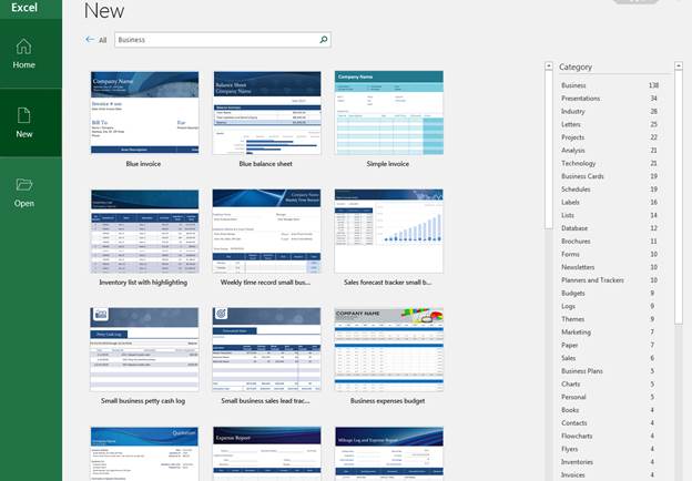
When you open Excel for the first time, you are shown a list of templates in the "Home" tab, but the "New" tab contains functionality to search for a specific type of template. For instance, you might want to create an invoice or receipt using Excel. You can find these templates in the "Business" category. Some templates fit into multiple categories, so you will find them in multiple categories during a search.
(New section of the opening window for Excel)
You can either click the link under the search bar or type a search phrase into the search text box and press "Enter." A list of templates is shown with additional categories on the right side of the window. These categories contain templates and can be used to search for the one that you need. Click another category name, and Excel will perform another search.
Double-click any template, and a new file is created with the template in place. When you create a new file with a template, just know that you aren't changing the actual template file. Template formulas, properties, styles and layouts are copied to a new Excel file and this file is independent from the Excel template file. Excel template files have the extension ".xltm" while a standard Excel spreadsheet file has the ".xlsx" extension.
Setting Up Custom Views
As you work with large spreadsheets, you'll need several columns and rows to store data. If you have several columns across a spreadsheet, some data might not be critical to what you're doing and having too many columns visible can make it so that you need to scroll and search data unnecessarily. You can hide columns and rows and save the new view as a stored custom view whenever you need to perform a certain task. Excel has features that let you save multiple custom views, so you can hide and show columns and rows with the click of a button. Any time you apply a certain custom view, you can always change it back to the Excel's "Normal" view, which is the default for each new spreadsheet that you create.
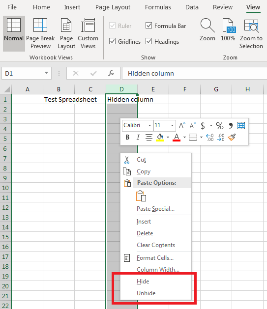
Custom views are unnecessary if you have no hidden columns and views, so the first step is to set up the columns and rows that you want to hide. The "Hide" and "Unhide" features are found in the context menu that displays when you right-click on a highlighted column or row.
(Hide and Unhide options)
You highlight an entire column by clicking the letter label at the top of the column. You can highlight an entire row by clicking the number at the left side of the spreadsheet row. After you highlight a column, right-click any highlighted section of the column. A context menu displays where you'll see a "Hide" and "Unhide" option at the bottom. Click "Hide" and the column and all of its data is no longer visible.
(Hidden column)
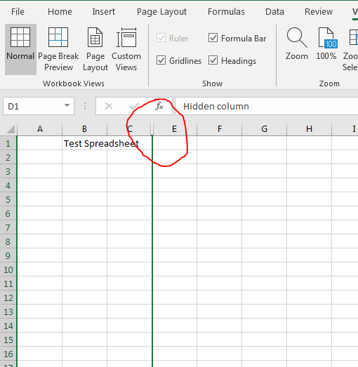
After the column is hidden, the letter is no longer seen at the top of the spreadsheet. When a spreadsheet is missing a letter in the alphabetic sequence, you know that it contains a hidden column.
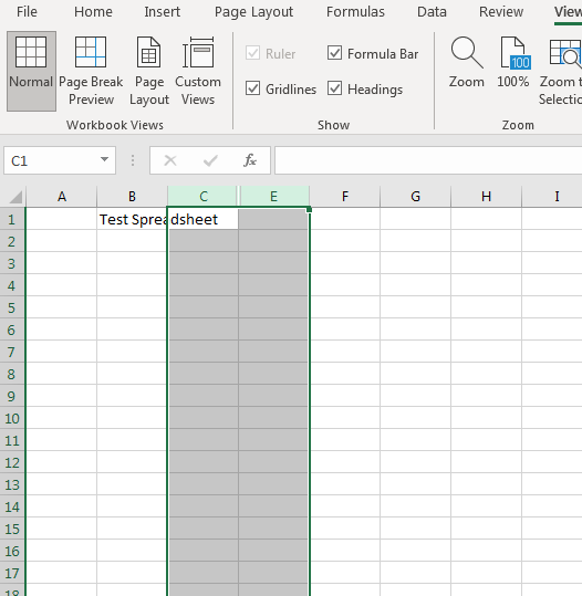
To unhide a column, you highlight the column to the left and the column to the right of it.
(Highlighted columns to unhide the hidden "D" column)
Right-click the highlighted columns and select "Unhide" to make the hidden column visible again. Since you want to create a custom view with the hidden column, re-hide the "D" column.
With the column hidden, you can now save this view. The first step is to click the "Custom Views" button in the "View" tab in the main Excel menu. The "Normal" and "Custom Views" buttons are located in the "Workbook Views" section.
When you click the "Custom Views" button, a window opens with a list of custom views. To add a new custom view, click "Add."
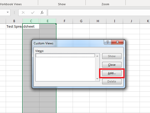
(Add new custom view)
After clicking the "Add" button, another window displays where you name your view. This name is what displays when you view a list of custom views that you can change or switch to.
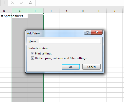
(Name custom view)
You also have the option to save print settings and any filters and settings. Type any name into the window and click "OK." Excel 2019 saves this view for future use.
At this point, you already have the "D" column hidden, so you don't need to switch to this view, but if you want multiple views with one that includes the hidden column, you should create a view with this column unhidden and save it. This would allow you to switch between a view that displays the "D" column and a view that hides it.
To activate a view, you need to select it from the list of custom views. Click the "Custom View" button to see a list of saved views. Select the saved view and click "Show."
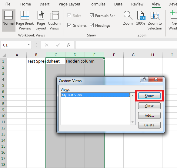
(Show and activate custom view)
Any hidden files, filter and print settings are activated when a custom view is shown.
Should you ever want to remove the custom view, click "Custom Views" again in the main menu, select the view that you want to delete, and click the "Delete" button.
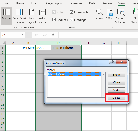
(Delete a selected view)
Ensure that you really want to delete a view before you remove it. If it's a view that hides or unhides columns or rows, you will have to manually make these changes after the view is deleted.
Cell Groups and Outlines
Many spreadsheets run totals and subtotals with grouped data. For instance, you might have a list of expenses for each month with subtotals at the bottom of your list to show the totals for a year. You can group this data either with totals that you've already added or have Excel add a subtotal for you.
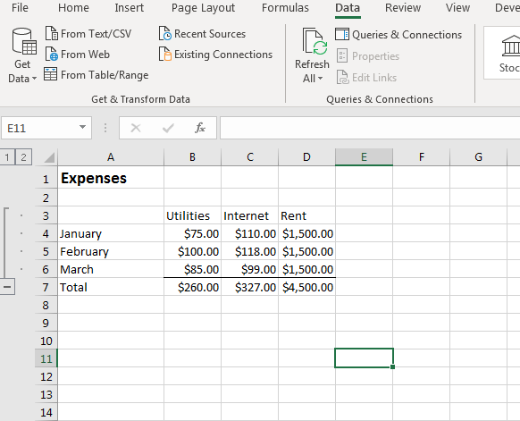
(Example grouped data)
The features to group data and create outlines can be found in the "Data" tab. The "Outline" section has three options: "Group," "Ungroup," and "Subtotal."
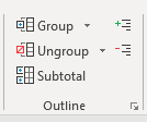
(Outline section of the "Data" tab)
The "Group" option groups data so that you can expand or collapse it. Similar to hiding and unhiding rows and columns, by grouping data you can expand or collapse it and only view subtotals. If you no longer need the data grouped, you can highlight it and click "Ungroup" to reverse the change.
You can use Excel 2019 functions to create subtotals at the bottom of a column or the far right of a row. For people who are unfamiliar with the way Excel functions work, you can let Excel create a subtotal section instead. This can be done by clicking the "Subtotal" button. You first need to select your data before you use any of these functions and set up preferences for changes to take effect.
Using the list of expenses for each month, highlight all data that you want to group. With rows and columns that have labels, you want to include these labels as well. With the data highlighted, click "Group." Do not include subtotals when you group data or subtotals will collapse and hide with the rest of the data. If you want the column headers to show when data is collapsed, then don't include these labels in your highlighted section.
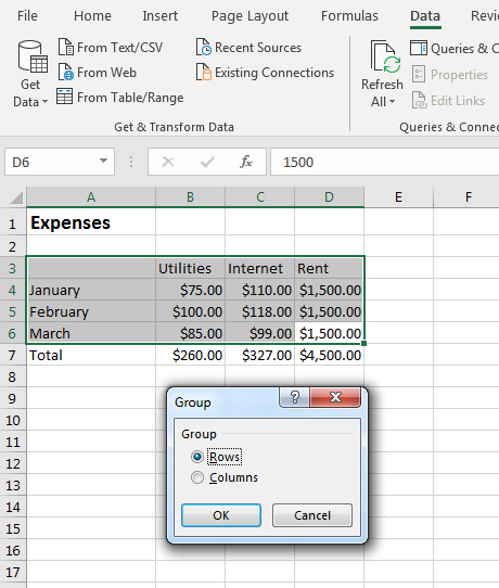
(Group options)
You can either group data by rows or columns. The way you group data will determine the way it's hidden and collapsed. For data that has a subtotal at the bottom of a column, grouping rows will collapse it so that only the subtotal shows. Select "Rows" and then click "OK" to apply changes.
Grouped data will show the option either above or to the left of it that lets you collapse it.
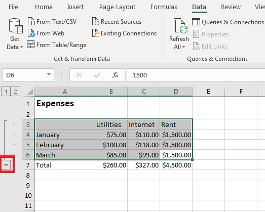
(Collapse button)
Click this button to hide the selected data. Click it again to expand it. Should you ever decide to ungroup the data, highlight it again and click the "Ungroup" data.
If you don't know how to use Excel functions for grouped data subtotals, you can let Excel do it for you before you set up data groups. Data groups with subtotals act slightly different than simple subtotals at the end of a column. Subtotals in data groups are used when you have multiple line items for each record. For instance, the "Utilities" section comprises gas, water and electric. You might want to separate these three costs and subtotal them. These subtotals would then be summarized at the end of a column into a grand total.
With the data detailed for the "Utilities" column, you can then highlight data that Excel will subtotal.
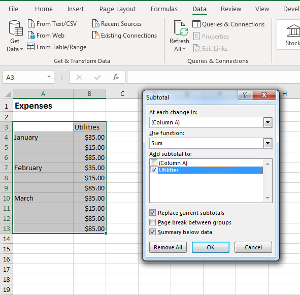
(Subtotal options)
The first column in this spreadsheet is the month. For each month, you need a new subtotal, so the "At each change in" option should stay at the default "Column A" selection. Since this column has no label, Excel automatically labels it "A" to give it some name. A subtotal is a sum of the detailed numbers, so the "Use function" should also stay at the default "Sum" selection.
The "Add subtotal to" section lists the columns that should be subtotaled. The selected data only has one column with data, so only one column is selected. The options under this section gives you additional ways to format your data such as add a page break after each subtotal or replace subtotals if you've already created them. After you've made your selections, click "OK" to apply them to the spreadsheet.
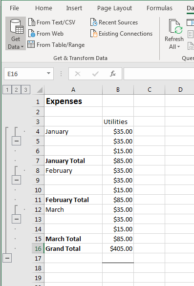
(Subtotals and Grand Total)
Notice that by subtotaling sections of your spreadsheet, it's automatically grouped and can be expanded and collapsed on each section. If you decide that you do not like the changes, you can click the "Undo" button to go back to the original version of your data.
Grouping and outlining are common on long spreadsheets with numerous data points. You can combine grouping with views so that you can toggle the data information that you view on large spreadsheets. For some common spreadsheets, you can probably find a template to use so that you don't need to create your own formulas and layouts.