
Importing Data Tables
Before you run queries on data, you need to either create your own data or import it from a data source. Part of the "Get & Transform" feature is to help you import data from a database source. Databases are much better at storing large amounts of data, so most Excel 2019 users will first need to import a table from a server database. The "Get & Transform" feature will help guide you through the process.
All data features for Excel are found in the "Data" tab. You can find import features in the "Get & Transform Data" section. Click the "Get Data" button, then click the "From Database" from the menu, then click "From SQL Server Database" in the submenu.
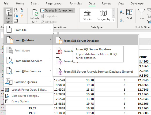
(Get data from database)
The menu option will open a configuration window. Before you can import a table from an external database, you need the username and password to access the database. You also need the name of the database and server address that stores the data. This information should be available from your network administrator.
Follow the prompts to enter database server information, and you are shown a list of tables stored in the database.
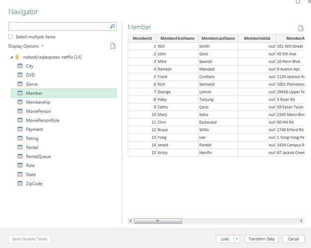
(Database tables)
For this example, a list of members will be imported into a new worksheet. Click the table name in the left panel, and Excel shows some of the data for review. Click the arrow next to the "Load" button and choose "Load To." This will allow you to configure the destination for the imported data.
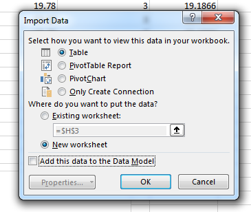
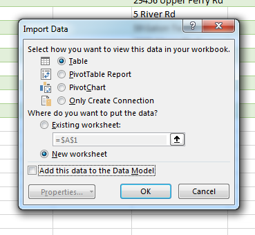
("Load To" configuration)
The default is "New worksheet," which is the best place to import data so that it isn't mixed with other sections of your data. Click the "OK" button to finish the import, and Excel 2019 loads data to a new spreadsheet.
Excel imports data exactly how it's stored in the source table, but it adds some formatting to it.
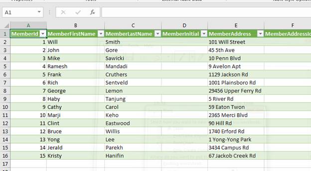
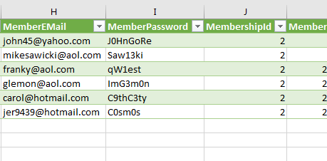
(Imported data worksheet)
With the table imported, you now have a complete snapshot of the information, but it does not give you analysis or reports on specific data. You can further segment the full table of data into smaller segments, and then run queries on the data to create reports. Excel has its own query tools to find the data that you need, move it to another worksheet (or section of the current worksheet), and then find data for further analysis.
Segmenting Your Data
The sample data is a list of members with their name and address stored in the "Member" table. It was imported in its entirety to an Excel worksheet. The "MembershipId" column contains an integer that indicates if the user has membership ID 1 or membership ID 2. Membership ID 2 is more expensive than 1, so you can segment a subset of data into another worksheet with only users that subscribed to membership ID 2. You do this using the "From Table/Range" feature.
This feature's button is also in the "Get & Transform Data" section of the "Data" tab.
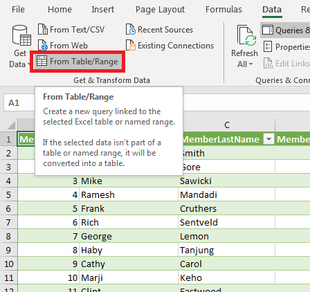
(From Table/Range button)
Before you open the Power Query editor, click a cell in the table to select it in the worksheet. Then, click the button, and a configuration window opens. This configuration window is Excel's Power Query editor. This editor is where you can query, transform, and edit data from your imported table.
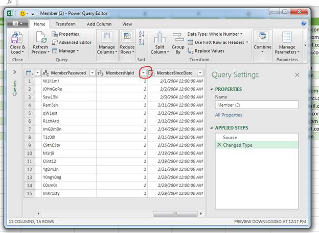
(Power Query editor)
The Power Query editor displays the data from your selected worksheet table. To the right of the header text, you'll find a dropdown arrow. Clicking this arrow displays a list of filter options. You can sort data, delete empty records, or use filter options to perform basic queries.
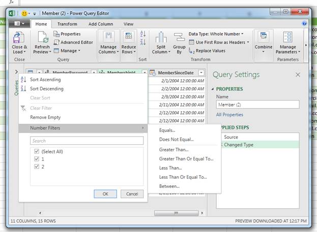
(Power Query filters)
By default, all records are selected. You can see the default filter in the bottom section of the menu where the "Select All" option is checked. Above this section is a search text box, or you can click the "Number Filters" option to open a submenu of conditional statements. Since the goal is to get a list of users with members ID 2, the "Equals" option is selected. A window then opens where you specify the value for your condition is entered.
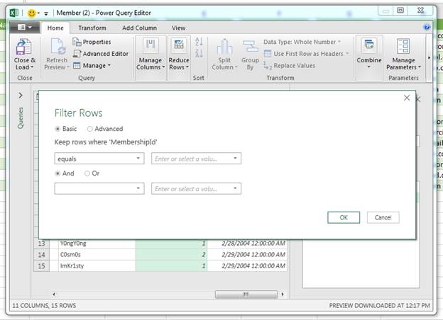
(Filter configuration window)
Because the "Equals" option was chosen, it's the default value selected in the first dropdown. To help you with choosing the right value, the dropdown to the right of the conditional statement contains the data stored in this column. Choose "2" from this dropdown.
Filter options include combination conditionals. The "AND" and "OR" statements let you add additional filter statements. There is an important logical difference between the two conditions. A mistake with these two statements can create the wrong results from your queries.
When you choose the "AND" condition, a record must match both statements for the record to display in results. If a record meets the first condition but not the second, it will be filtered out of the result set. If you choose the "OR" condition, a record only needs to meet just one of the conditions for it to be included in the result set.
Excel doesn't require you to set an additional statement. If you only want one statement to filter records, ignore the section dropdown sections and click "OK" to run the filter query.
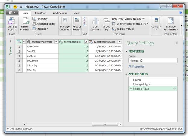
(Power Query results)
The results display in the Power Query editor. You can see that only user records with a membership ID of 2 are shown. Should you forget if the records shown are filtered, you can look in the "Applied Steps" section to see that it includes "Filtered Rows." If you want to remove this filter, click the "X" icon next to the label. If you want to change the filter parameters, click the gear next to the label and the filter configuration window opens again.
Suppose now that you want to search for a particular user stored in the filtered data results. You can either remove the filter or perform a search on filtered, segmented data. For this example, a search for a user by last name will be performed. Scroll to the "MemberLastName" column and click the filter dropdown arrow.
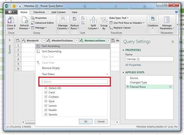
(Search filter)
You could perform another filter similar to the previous one by using the "Equals" condition to enter a name, or you can use the search text box. Enter "Lemon" in the search text box to find a user with the last name of "Lemon" in the data set.
The advantage of using the search is that you can get a quick view of results without applying filters to the table.
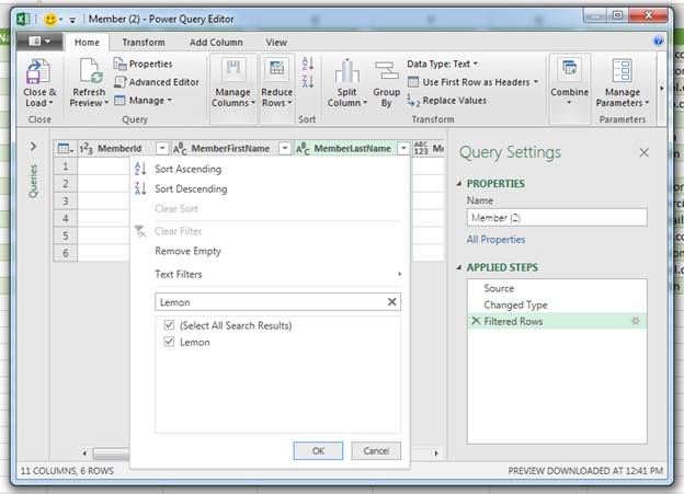
(Search results)
Searching for a record using this method will show you results in the filter menu. Click the "X" icon in the search text box to clear the filter or click "OK" to apply results in the Power Query editor. For this example, click "Cancel" to avoid applying the filter and return to the main Power Query editor view.
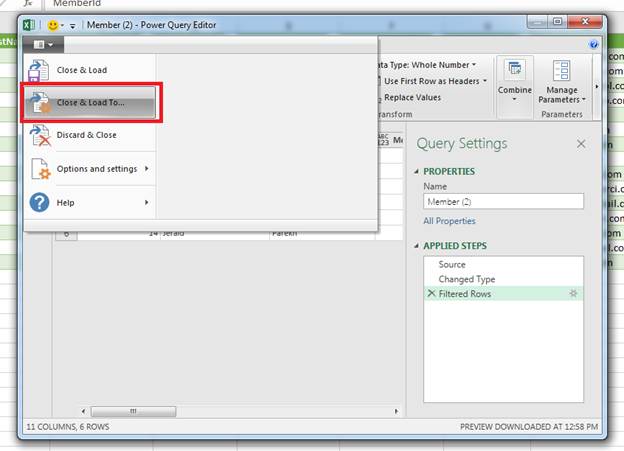
With the new subset of data, you can now create a new worksheet so that you have a new table with just the data that you want to work with. Click the "Options" dropdown in the upper-left corner of the main window and choose "Close and Load To" to open a window where you configure the destination location.
(Close and Load To)
You can also close the current table and load another, or just discard the filter changes and close the Power Query window. The "Close and Load To" option saves the subset of data so that you can work with it further. Click this option and Excel prompts you for a destination location.
(Load To configuration)
For this example, the subset of data will be stored in a new worksheet. Leave the default option selected (New worksheet) and click "OK" to move the data into a new worksheet. The query runs and moves data to a new worksheet, and now you have only members with a membership ID of 2.
(Exported filtered data)
With this new subset of data, you can re-open the Power Query editor to query and edit your data. Power Query isn't only restricted to filtering data. You can also edit and change the way your data is structured as well as the table itself.
Editing Tables and Data
After creating a subset of data, you can use the Power Query editor to set up columns, edit data, and run formulas on it. Click the new table, and then click the "From Table/Range" button to open Power Query. Click the "Add Column" tab. This tab is where you can add a new column and set its properties to include additional information.
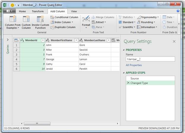
(Add column tab)
The right side of the menu lets you define the type of column that you want to add, but sometimes you don't know the data type that should be defined. When you define a data type for a column, you're restricted to entering only this type of value. You can get around limitations in Excel 2019, but should you decide to export the data from the worksheet to an existing database table, you could have issues exporting and the database throws you an error.
If you are unsure of the type of data that you want to store in the column, you can use one of the features in the "General" section of the main menu. Click the "Column from Examples," and you can enter the type of data that you plan to store, and Excel will detect the data type and create a column based on your input.
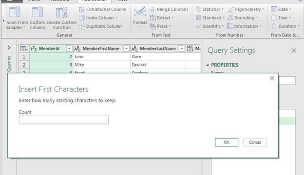
To extract data, first click the "MemberFirstName" column. Next, click the "Extract" button in the "From Text" section and choose "First Characters" to open a configuration window. This option lets you extract a number of characters from a text column. For instance, you might want to get the first initial from a member's first name and then create a column based on the results. The features in the "From Text" section use characters from text columns to create a new column. The "From Number" section extracts information from numeric columns. The "From Date" section extracts data based on date columns.
(Extract characters configuration)
The configuration prompts depend on your choice of data extraction. Since the "First Characters" option was chosen, a window opens prompting you for the number of characters that you want to extract. The goal is to get just the first initial of the first name, so enter "1" and then click "OK" to apply the changes.
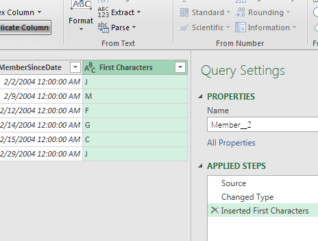
(Extracted column data)
You can see from the results that a new column is created named "First Characters" filled with the first initial of the member's first name. The "Applied Steps" shows that an additional change was made to the table so that you can delete it or edit the data.
Excel provides a default name for the column but leaving the column as "First Characters" doesn't describe the data. It's best to change the column header to one that properly explains that it's the first initial of the user's first name. You can change column headers by right-clicking the column and selecting the "Rename" option.
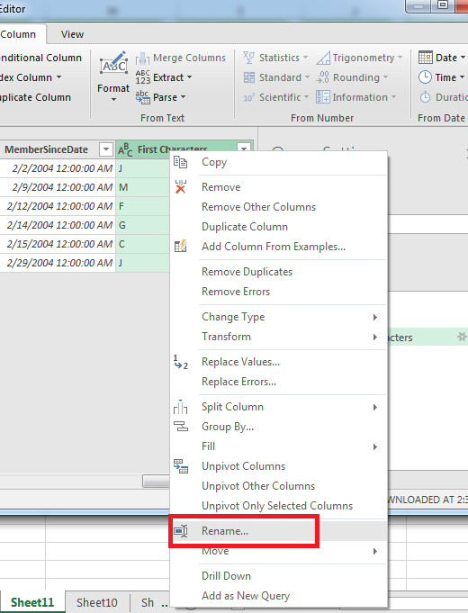
(Column context menu)
The context menu when you right-click a column has several formatting and data manipulation options. After clicking the "Rename" menu option, the column header text is highlighted, and you can now enter a new name for the column. Type a new header name for the column and press "Enter." The new name is now the header text for the column. If you export this data set to a new worksheet, the column name will be used.
The Power Query editor has numerous more options for you to create, edit and delete data from a subset of information stored in your worksheets. Use this tool when you have a large table of data that can be used to create reports and run analysis on only a subset of information. By creating these data subsets, you can improve analysis speed and work with just the data that you need.