
Set Up the List
Before you create a dropdown list in Excel, you need a list of data to use. Since you can make multiple worksheets in one Excel workbook, most people use a separate sheet to populate the data list. You can then configure any specific cell in the Excel form to point to this list of data. You then set the cell as a list, and Excel does the rest for you.
You don't have to use a separate sheet to populate a data list. You can use the same sheet or even a separate workbook. You can use a separate workbook, but any changes to this workbook could affect the data list. Also, if the workbook is moved to a different directory or storage location, your list will no longer function.
For simplicity, this article's examples use the same workbook and worksheet, but just know that you can use references to separate worksheets and workbooks for your own data lists.
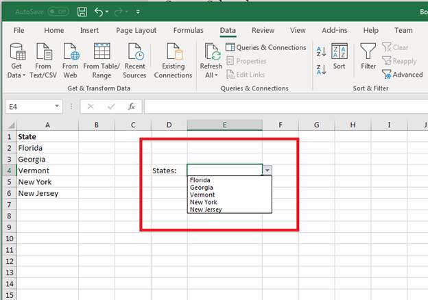
Create a blank worksheet in a currently opened workbook, or you can create a new workbook to store the new data list. In the following scenario, a list of states is used for a data list. We'll add five states to the first column (A) in a new worksheet.
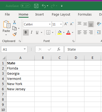
(List of states set up for a dropdown)
In the image above, five states were added to their own cells. Notice at the top that "State" is used to label the column list. This is beneficial for the dropdown that we'll make, and it helps label data so that others can understand what the list is used for. The list can be as long as it needs to be, but we've only added five states for simplicity.
You now need a place to display the dropdown that will contain these values. For simplicity, we'll set up a dropdown in the same worksheet. Make sure that you label the dropdown as well so that users know what the dropdown list is for.
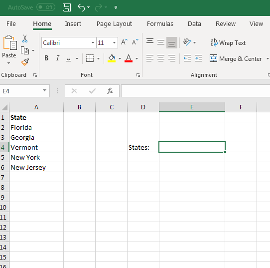
(Location of the state dropdown and its label)
In the image above, the cell E4 is selected as the cell that will contain the dropdown list. In D4, the label "States:" is displayed so that users know a list of states will be shown in the dropdown. It also helps users understand that they must select a state when they fill out the form. Labeling cells is an important part of creating effective spreadsheets that store the right data, especially among several users that add data and revise it periodically.
Creating a Dropdown Based on External Data
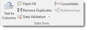
With the cell next to the "States:" label selected, click the "Data" tab. The "Data" tab has several data tools that you can use to work with lists. Click the "Data Validation" button, which is found in the "Data Tools" section of the "Data" tab.
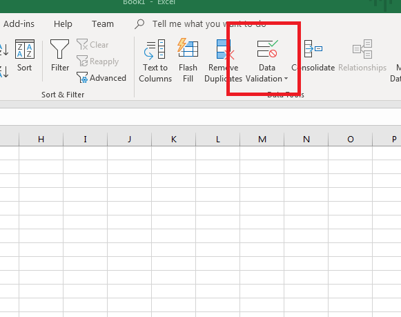
(Location of the "Data Validation" button)
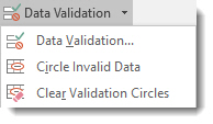
Clicking this button displays another dropdown selection. Click the "Data Validation" option, and a new window opens where you can configure your data list and cell that contains the options for a user to choose from.
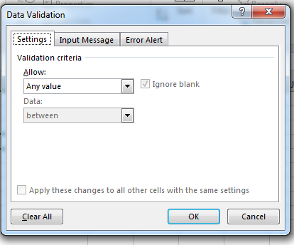
(Data validation configuration window)
In the window above, you have several options to set a dropdown using a list of data. For a dropdown, you need to choose the "List" option. The "List" option is found in the "Allow" dropdown box.
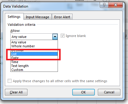
(Select "List" for the validation criteria)
In the image above, notice that the "Allow" dropdown has the "List" option selected. This option tells Excel 2019 that you want to use a data list. If you hadn't already created a data list in an external workbook or in a worksheet in the current workbook, you would need to cancel out of this window and create a list. For this reason, it's better to create a list of data that you want to display in a dropdown before setting up this configuration option.
When you select "List" from the dropdown, a new list of options display in the "Data Validation" window. The "Source" text box is where you can type the range of cells. With a list of only five states, it's easy to take a look at the cells that contain states and type them into this text box. However, when you have a range of cells that span several rows, you'd have to scroll down the spreadsheet to find the last cell in the list. You could also have empty cells that you miss as you scroll down the list. Instead of typing the cell range manually, you can click the arrow up button adjacent to the "Source:" text box. This opens a view of your spreadsheet where you can use your mouse to select the cells that contain a list of data.
Click the arrow button next to the "Source" text box to trigger the data selection feature. The "Data Validation" window collapses and then only the Source text box displays. Use the mouse to highlight each state. You don't need to click the states individually. Instead, click the first state and drag your mouse to the last state in the list. The data validation tool will automatically create the range in the text box with the right textual labels that reference cells containing the information to display in the dropdown.
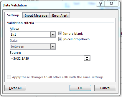
(Data list selected and displayed in Source text box)
Click the "Input Message" tab to see a list of options to prompt the user with information when the input cell is selected. In some scenarios, having a label such as "State" is not enough to explain what the user should input. You might need additional information to explain what is needed using a prompt. You could set a Note but these notes are used for revisions and not the best option for setting instructional information. With an Input Message, you can prompt the user and display additional information when the cell is selected.
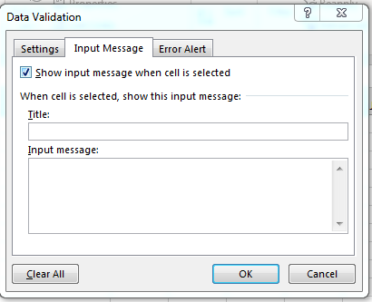
(Input message configuration window)
The input configuration window contains a title and an input message. The "Title" text box is where you set up the main title that the user will see when clicking the cell. The "Input Message" is arguably the more important input text box. This text box describes the purpose of the input selected by the user. It gives additional information to help the user understand the right data selection when filling out the Excel 2019 form.
Fill out these two input fields if you think more information is needed for the user as the form is filled out. Click the "Error Alert" tab to set up an error message or warning for the user should one occur.
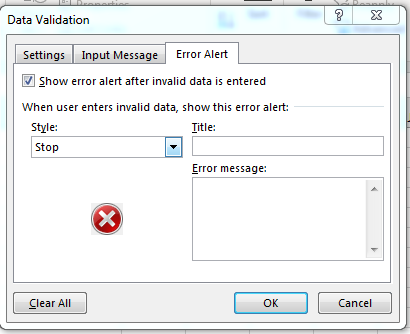
(Error alert option for a data dropdown)
In the configuration window above, the check box labeled "Show error alert after invalid data is entered" tells Excel to stop the user and display the configured error should the user enter invalid input. For instance, we have five states from which the user can select in a dropdown. If the user decides to enter a state that isn't in the list, then Excel would display an error and prompt the user to re-enter information to valid input. You can remove this selection to skip the option, but you should only skip this option if you do not want to restrict data entry to only what's available in the dropdown list.
In the "Style" dropdown, you can choose if you want to stop the user (the default), or if you want the message to show as an informational note or a warning. This gives you granular control of invalid data errors, so that you can choose if you want to allow the user to continue filling out the form even if data is incorrectly entered.
The "Title" and "Error message" input boxes are the text displayed to the user. Just like the 'Input Message" option, the "Error message" text box is the most important because it gives the user detailed information on why the input is invalid.
After you make your choices in all three tabs, click the "OK" button, and Excel 2019 sets up the dropdown list in the selected cell.
(Dropdown using a data list)
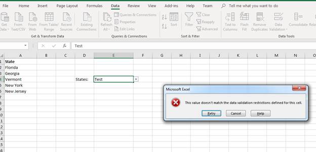
You can test the new dropdown data list by selecting data. You can also test the error messages by setting the cell to a state that does not match one in the set list.
For instance, first click the arrow in the dropdown and select "Florida." Notice that no error message is displayed. Next, click the dropdown cell, which is E4 in this example. Type the word "Text" in the input cell. Click away from the input cell by clicking cell F1. Notice that an error message displays indicating that incorrect input was detected.
(Error message displayed from invalid input)
This error and validation control let you stop invalid input so that you can keep a spreadsheet of data that follows a strict rule set. By blocking invalid input, you can ensure that only a specific set of data is added to your input forms.
Dropdown lists are a common part of forms, and Excel makes it easy to create them whether the list contains 2 or 2000 cells. Dropdown lists are valuable when you have a set list of items from which you want users to choose, so they cannot just type any value into a cell. Using data lists makes creating long forms with multiple dropdown lists faster and remember that you aren't limited to just the current sheet. You can reference any worksheet or workbook that contains your data by just adding the appropriate reference syntax in your data validation options.
Managing Data
Most people who are familiar with the MS Office suite associate complex forms with Excel's sister program Access, but you can use them in Excel as well. In fact, you can even share data between the two programs.
There are two kinds of forms available in MS Excel: data forms and worksheet forms.
-
Data forms are generally used for data entry. They are simple forms that list the contents of a single column. What's more, they can display up to 32 fields at a time. This is especially helpful when dealing with a data range that reaches across more columns than will fit on a screen. You can insert, alter, delete, and even find records with data forms.
-
Worksheet forms are more sophisticated and specialized. They can be customized to fit the information at hand or to fill a particular need. They can even be complex and appealing enough to be printed or distributed online. Worksheet forms must be created using the Microsoft Visual Basic Editor.
Adding the Form Button to the Quick Access Toolbar
The Form button is not included in the ribbon, but you can add it to the Quick Access Toolbar, which, if you remember, is in the upper left hand corner of the application window.
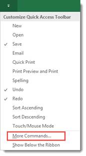
To add the Form button, click the arrow to the right of the Quick Launch toolbar and select More Commands. This will launch the Excel Options window, which can also be accessed by clicking Options on the File tab.
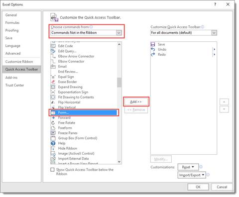
In the "Choose commands from" box, select Commands Not In the Ribbon, then scroll down through the list until you find Forms. Select it and click Add. When you are finished, click OK.
This is what the Form button looks like:  .
.
Adding Records Using the Data Form
When you click the Form button for the first time, Excel will analyze the row of field names and entries for the first record. It uses that information to create a data form.
Let's click on the Form button now.
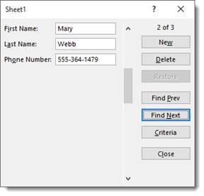
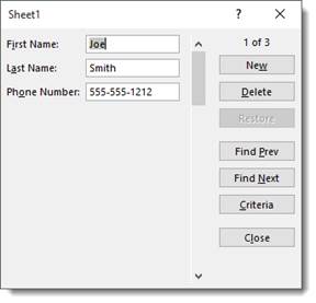
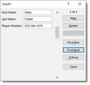
The first record appears in the dialogue box:

Click Find Next to find the next record.
If you want to add a new record using the data form, click New.
As you can see in the snapshots above, the number of the record appears above the New button.
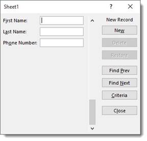
However, when you click the New button, it lets you know that it's a new record.
Let's add a new record.
Enter the information, then hit Enter.
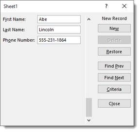
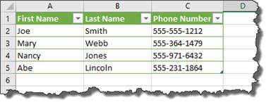
The new record appears in your list:
You can hit ESC when you're done adding records.
Editing Records in the Data Form
In addition to adding records, you can also edit them. You can use the data form to find records that need updated or removed from the list.
To do this, click the Form button on the Quick Access Toolbar.
Find the record that you want to update or remove.
Now click in any of the fields to update the data. You can also delete data in the field.
Hit Enter.
Navigating Through Records in the Data Form
If you have a lot of records, navigating through them can be a challenge. The data form makes it a bit easier.
If you want to move to the next record in the data form, press Enter or the down arrow key.
To move to the previous record, hit the up arrow or press Shift+Enter.
To move to the first record in the data list, press CTRL+ ? (up arrow) or press CTRL+PgUp.
To go to a new data form that comes after the last record, press CTRL+ ? (down arrow) or CTRL+PgDn.
Find Records in the Data Form
If you want to find a specific record, you can use the Criteria button in the data form. It's pictured below.
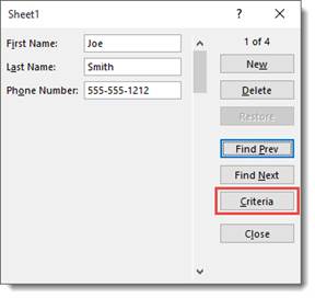
When you click the Criteria button, Excel 2019 clears the field entries in the data form. Instead, the word Criteria is displayed.
Let's push the Criteria button to show you what we mean.
We now see a blank data form.
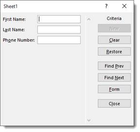
Notice that the word Criteria is above the new button, and the new button is inactive since we're searching for a record.
Now, let's say you're looking for a woman named Mary Webb, but you have 5000 women named Mary in your list.
Enter the criteria: Mary Webb.
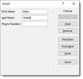
Now click the Find Next button.
As you can see, it brings up the record.
You can also include the following operators in search criteria to help you find the record you need:
-
? for single
-
* for multiple wildcard characters
-
= Equal to
-
> Greater than
-
< Less than
-
>= Greater than or equal to
-
<= Less than or equal to
-
<> Not equal to
Data Validation
Data Validation lets you choose what information is acceptable to enter into a cell. For instance, you may have a product code that has four digits. You can set up a cell so that anything other than a 4-digit number will display an error message.
To set up data validation, select a cell or cells, then click the Data tab. Go to Data Validation in the Data Tools group.
Choose Data Validation from the dropdown menu.
You'll see this window:
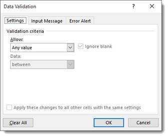
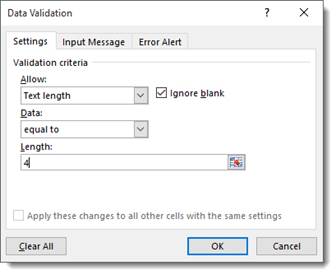
Since we're going to set up a cell to accept only a 4-digit number, we will select Text length from the drop down menu that says "Allow" over it. From the Data dropdown menu, we are going to select "equal to" and in the length text field we will type "4." That tells Excel we want an entry with four characters.
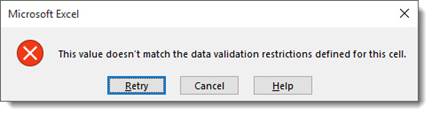
From here, we can hit OK and have Excel 2019 provide a generic warning that looks like this:
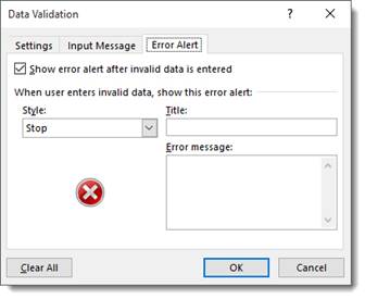
Alternatively, we can create a custom warning by selecting the Error Alert tab. Which looks like this:
Here we have selected the Warning style and entered the text for our error alert.
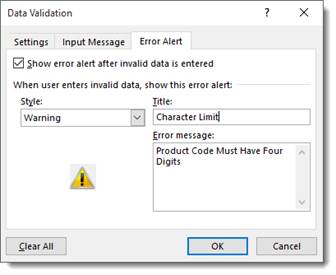
When a user enters a code of less or greater than four digits, the message will look like this:
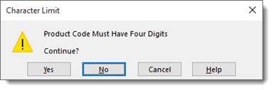
There are three kinds of error messages available in Excel: information messages, warning messages, and stop messages. Information messages and warning messages do not prevent invalid information to be entered into the cell; they simply inform the user that such an entry has been made. Users can choose to ignore the warning. A stop message, on the other hand, will not allow an invalid entry. It has two buttons, Cancel and Retry. Cancel restores the cell to its original value, and retry returns them to the cell for further editing.
You can also set up a message to remind users what the restrictions or expectations are. Use the Input Message tab to create a custom reminder.
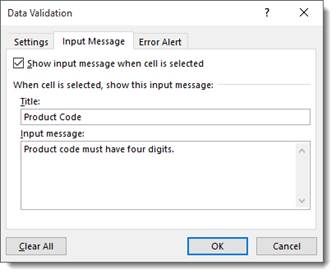
It will display anytime the cell or the range of cells is selected, as in the example below.
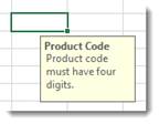
Auditing
MS Excel gives you a variety of tools to audit information in a worksheet. Just like data forms, formula auditing can take some of the confusion and frustration out of dealing with lots of different formulas. You can also see which cells have invalid information in them.
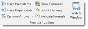
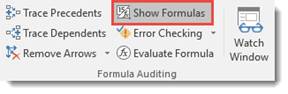
To use these tools, go to the Formulas tab, then the Formula Auditing group.
Select Error Checking and choose Error Checking from the dropdown menu.
That said, it is not always apparent which cells have formulas in them. Therefore, the first step to evaluate the formulas is to find them. Click the Show Formulas button, as highlighted below.
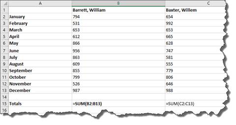
As you can see in the example below, the whole numbers will be changed to the formulas and the formula cells will be selected.
To make it easier to see the cells when they are no longer selected, you can click the fill  button. This will fill the selected cells with very visible yellow.
Let's take a closer look at the other functions in the Formula Auditing group.
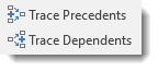
These two buttons allow you to trace (and turn off trace) precedents in a formula. A precedent cell is one that is referred to by a formula in another cell.
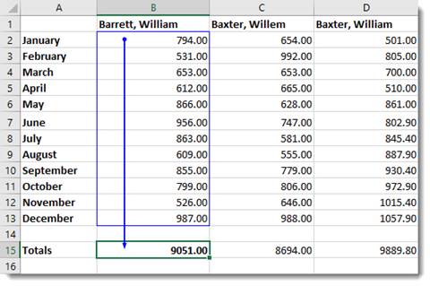
B2 thru B13 are precedents because they are referred to in the formula in cell B15. As you can see, the trace precedents button shows you the relationship between the cells.
The next button removes all arrows. 
The Watch Window (pictured below) is useful when you're not sure if alterations to the value in a cell will affect a formula. You can easily remind yourself of the formula by adding it to the watch window.

The Evaluate Formula function will perform the calculations of a formula in slow motion so you can see each step. To use it, select a formula, then click the Evaluate Formula button  in the toolbar. You will see a box that looks like this:
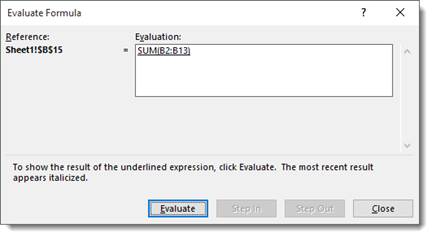
Click the Evaluate button to see Excel 2019 perform the calculations in slow motion. Use the Step In and Step Out buttons to navigate through each step in the formula.
Introduction to Data Plotting Using 3D Maps
Excel lets you explore your data in a worksheet by plotting it on a map. For example, you might want to create a 3D map to show the cities where your customers live. You will need an image of a map in either .jpg, .png, or .bmp format. If the data you wish to plot on a map doesn't relate to cities, but perhaps instead locations in a warehouse, you'll want to upload an image that relates to your data. That said, you will also need data that relates to the picture so that your data can be plotted using an XY coordinate system.
To create the 3D map, go to the Insert tab, then click the 3D Map button.

It may take a moment to load, but you will see the 3D Map screen.
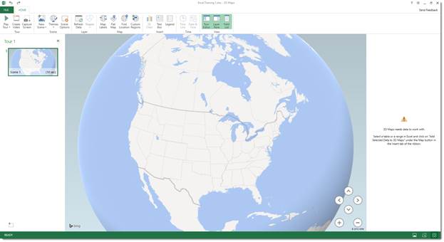
To create a map customized for your data, click New Tour.
Go to Home>New Scene in the 3D Map screen.
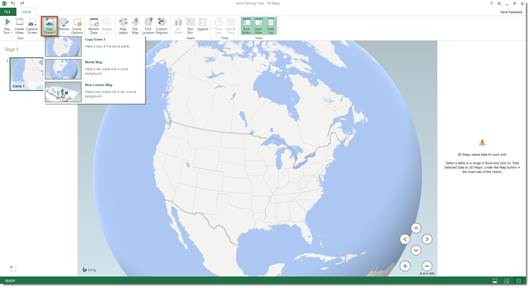
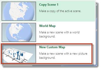
From the dropdown menu, select New Custom Map.
You will then see this dialogue box:
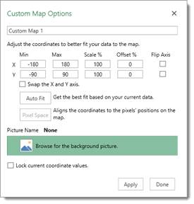
Locate the background picture you want to use.
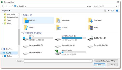
Click Open.

You can now see your picture open in the 3D Map window. Use the dialogue box to adjust the XY coordinates if needed.
Click Apply, then Done.